Understanding EIGRP – Part 2
Dec 02, 2016

In the first blog post in our Understanding EIGRP series, we were introduced to EIGRP’s features, in addition to a basic configuration example, and a collection of verification commands. Now, in this post, we’ll delve into the behind the scenes action of how EIGRP establishes a neighborship, learns a route to a network, determines what it considers to be the best route to that network, and attempts to inject that route into a router’s IP routing table.
EIGRP’s operations can be conceptually simplified into three basic steps:
Step 1. Neighbor Discovery: Through the exchange of Hello messages, EIGRP-speaking routers discover one another, compare parameters (for example, autonomous system numbers, K-values, and network addresses), and determine if they should form a neighborship.
Step 2. Topology Exchange: If neighboring EIGRP routers decide to form a neighborship, they exchange their full topology tables with each other. However, after the neighborship is established, only changes to the existing topology are communicated between the routers. This approach makes EIGRP much more efficient than a routing protocol such as RIP, which advertises its entire list of known networks at regular intervals.
Step 3. Choosing Routes: Once an EIGRP router’s topology table is populated, the EIGRP process examines all learned network routes and selects the best route to each network. EIGRP considers a network route with the lowest metric to be the best route to that network.
As you read the following discussion detailing EIGRP neighbor discovery, topology exchange, and route selection, please keep in mind that unlike OSPF, EIGRP has no concept of a Designated Router (DR) or Backup Designated Router (BDR), which you might have learned about in your CCNA R/S studies.
Neighbor Discovery and Topology Exchange
To better visualize how an EIGRP router discovers its neighbors and exchanges topology information with those neighbors, consider the figure below.
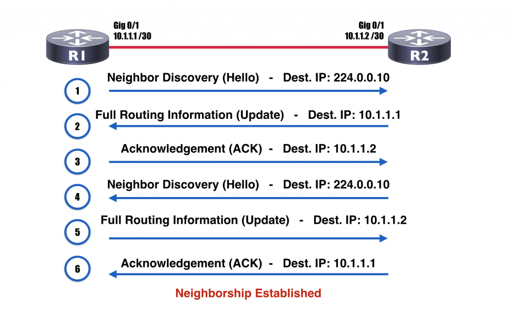
The six steps depicted in figure above perform as follows:
Step 1. Router R1 wants to see if there are any EIGRP-speaking routers off of its Gig 0/1 interface with which it might possibly form a neighborship (also known as an adjacency). So, it multicasts an EIGRP Hello message to the well-known EIGRP multicast address of 224.0.0.10 asking for any EIGRP-speaking routers to identify themselves.
Step 2. Upon receipt of router R1’s Hello message, router R2 sends a unicast Update message back to router R1’s IP address of 10.1.1.1. This Update message contains router R2’s full EIGRP topology table.
Step 3. Router R1 receives router R2’s Update and responds with an Acknowledgement (ACK) unicast message sent to router R2’s IP address of 10.1.1.2.
Step 4. The process then repeats itself with the roles reversed. Specifically, router R2 sends a Hello message to the EIGRP multicast address of 224.0.0.10.
Step 5. Router R1 responds to router R2’s Hello message with a unicast Update containing router R1’s full EIGRP topology table. This Update message is destined for router R2’s IP address of 10.1.1.2.
Step 6. Router R2 receives router R1’s routing information and responds with an ACK unicast message sent to router R1’s IP address of 10.1.1.1.
At this point, an EIGRP neighborship has been established between routers R1 and R2. The routers will periodically exchange Hello messages, to confirm each router’s neighbor is still there. However, this is the last time the routers exchange their full routing information. Subsequent topology changes are advertised via partial updates, rather than the full updates used during neighbor establishment. Also, notice that the Update messages during neighbor establishment were sent as unicast messages. However, future Update messages are sent as multicast messages, destined for 224.0.0.10. This helps ensure all EIGRP-speaking routers on a segment receive the Update messages.
EIGRP boasts an advantage over OSPF in the way it sends its Update messages. Specifically, EIGRP’s Update messages are sent reliably using Reliable Transport Protocol (RTP). This means that, unlike OSPF, if an Update message is lost in transit, I will be retransmitted.
NOTE: The acronym RTP also refers to Real-time Transport Protocol (RTP), which is used to transmit voice and video packets.
Route Selection
The routes shown in an EIGRP topology table include metric information, indicating how “far” it is to a specific destination network. But just how is that metric calculated? Well, EIGRP’s metric calculation is a bit more involved than with RIP or OSPF. Specifically, EIGRP’s metric is an integer value based on bandwidth and delay, by default. Although, its metric calculation can be include other components. Consider EIGRP’s metric formula:
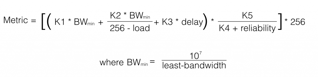
Notice the metric calculation involves a collection of K-values, which are constants you can configure to be zero or some positive integer. The calculation also considers bandwidth, delay, load, and reliability. Interestingly, much of the EIGRP literature states that the metric is also based on an interface’s Maximum Transmission Unit (MTU). However, you can see from the metric calculation formula, MTU is conspicuously absent. So, what’s the deal? Does EIGRP consider an interface’s MTU or not?
When EIGRP was originally designed, the MTU was designated as a tie breaker if two routes had the same metric but different MTU values. In such a situation, the route with the higher MTU would be selected. So, while an EIGRP Update message does indeed contain MTU information, that information is not directly used in metric calculations.
Next, let’s consider each of the different components of EIGRP’s metric calculation, and the tiebreaking MTU:
- Bandwidth: The bandwidth value used in the EIGRP metric calculation is determined by dividing 10,000,000 by the bandwidth (in kbps) of the slowest link along the path to the destination network.
- Delay: Unlike bandwidth, which represents the “weakest link,” the delay value is cumulative. Specifically, it’s the sum of all delays associated with all of the interfaces that must be exited in order to get to the destination network. The output of the show interfaces command shows an interface’s delay in microseconds. However, the value used in EIGRP’s metric calculation is in tens of microseconds. This means you would add up all of the egress interface delays as seen in the show interfaces output for each egress interface, and then divide by 10 to get the tens of microseconds unit of measure.
- Reliability: The reliability is a value used in the numerator of a fraction, with 255 as its denominator. The value of the fraction indicates the reliability of a link. For example, a reliability value of 255 indicates the link is 100 percent reliable (that is, 255/255 = 1 = 100 percent).
- Load: Similar to reliability, load is a value used in the numerator of a fraction, with 255 as its denominator. The value of the fraction indicates how busy a link is. For example, a load value of 1 indicates the link is minimally loaded (that is, 1/255 = 0.004 < 1 percent).
- MTU: Although it doesn’t appear in EIGRP’s metric formula, an interface’s MTU value (which defaults to 1500 Bytes) is carried in an EIGRP Update message to be used in the event of a tie (for example, two routes to a destination network have the same metric but different MTU values), where the higher MTU value is preferred.
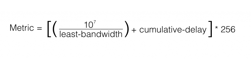
As a memory aid, remember the acrostic Big Dogs Really Like Me. The B in Big can remind you of the B in Bandwidth. The D in Dogs can remind you of the D in Delay, and so on. However, by default, EIGRP has most of its K-values set to zero, which dramatically simplifies the metric calculation to only consider bandwidth and delay. Specifically, the default K-values are:
K1 = 1
K2 = 0
K3 = 1
K4 = 0
K5 = 0
If we plug these default K-values into the EIGRP metric calculation, the value of each fraction equals zero, which reduces the formula to:
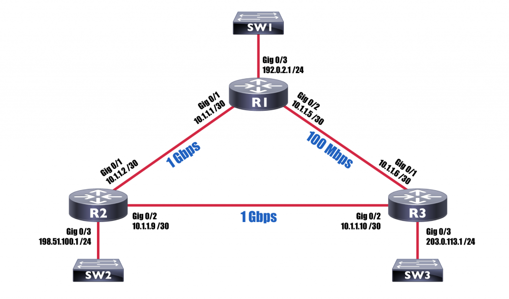
To further reinforce this concept, let’s do a metric calculation, and see if it matches our EIGRP topology table. Consider the topology shown in the figure below.
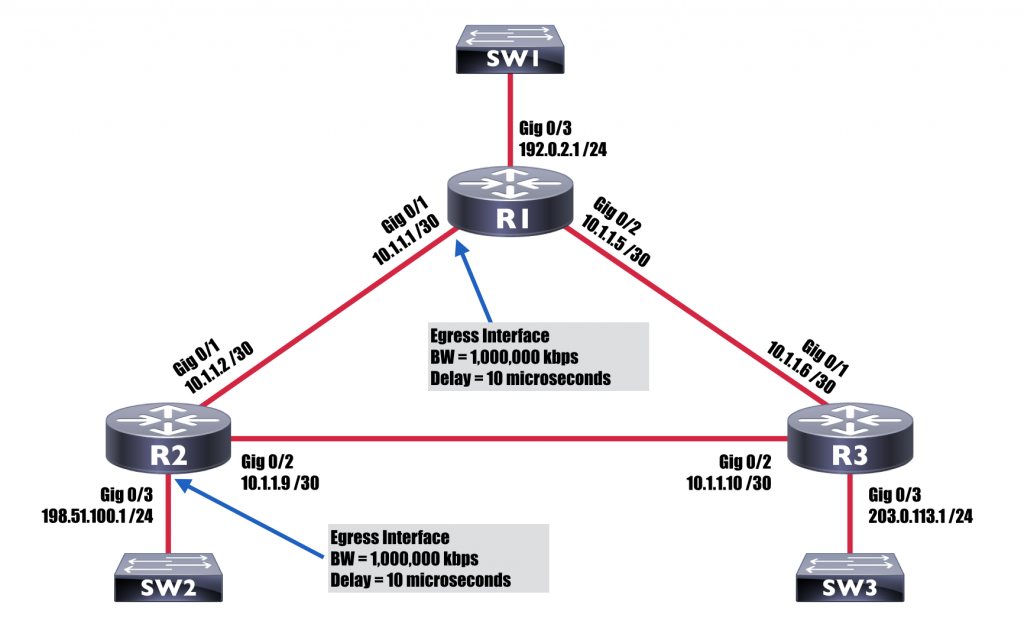
Suppose we wish to calculate the metric to the 198.51.100.0 /24 network from the perspective of R1 for a route that goes from R1 to R2 and then out to the destination network. From the topology, we can determine that we’ll need to exit two router interfaces to get from router R1 to the 198.51.100.0 /24 network via router R2. Those two egress interfaces are interface Gig 0/1 on router R1 and interface Gig 0/3 on router R2. We can determine the bandwidth and delay associated with each interface by examining the output of the show interfaces commands given in following example.
Determining Interface Bandwidth and Delay Values on Routers R1 and R2
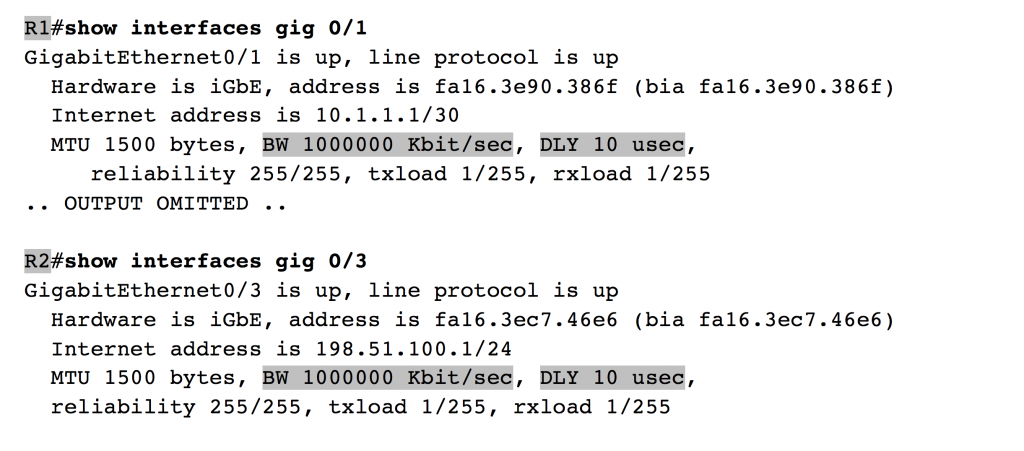
From the above example, we determine both egress interfaces have a bandwidth of 1,000,000 kbps (that is, 1 Gbps). Additionally, we see that each egress interface has a delay of 10 microseconds. The bandwidth value we plug into our EIGRP metric formula is the bandwidth of the slowest link along the path to the destination network, as measured in kbps. In our case, both egress interfaces have the same link speed, meaning that we say our “slowest” link is 1,000,000 kbps.
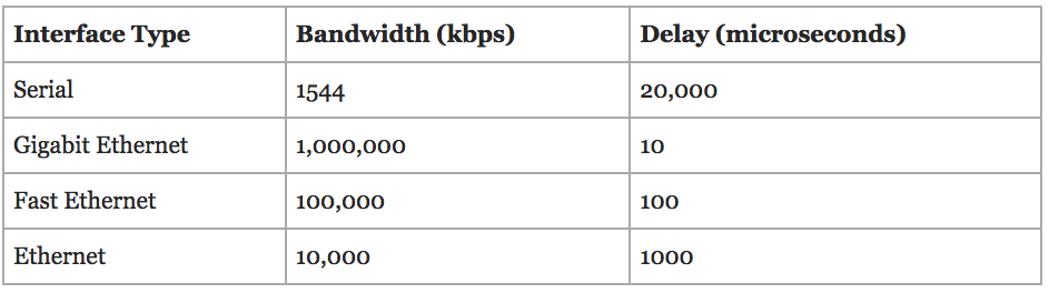
As a reference, the tale below shows common default values for bandwidth and delay on a variety of Cisco router interface types.
Common Defaults for Interface Bandwidth and Delay
Our delay value can be calculated by adding up the egress interface delays (as measured in microseconds) and dividing by 10 (to give us a value measured in tens of microseconds). Each of our two egress interfaces has a delay of 10 microseconds, which gives us a cumulative delay of 20 microseconds. However, we want our unit of measure to be in tens of microseconds; so we divide 20 microseconds by 10, which gives us 2 tens of microseconds. We now have the two required values for our formula: Bandwidth = 1,000,000 kbps and Delay = 2 tens of microseconds. Now, let’s plug those values into our formula:
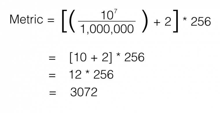
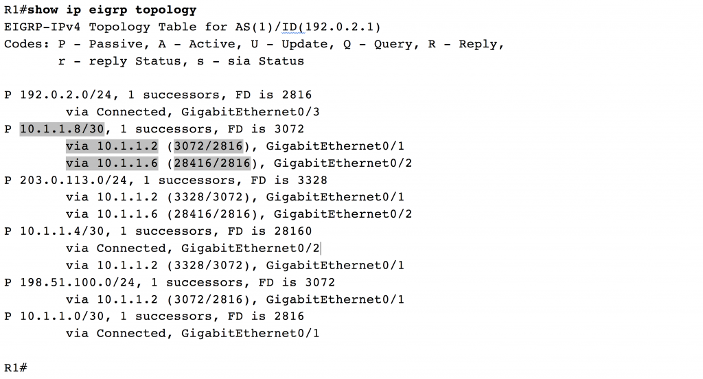
Our calculated EIGRP metric value is 3072. Now, let’s see if that’s the actual metric appearing in router R1’s EIGRP topology table. Output from the show ip eigrp topology command issued on router R1 is shown in the following example.
Checking the EIGRP Metric for Network 198.51.100.0 /24 on Router R1
As predicted, the metric (also known as the feasible distance) from router R1 to the network of 198.51.100.0 /24 via router R2 is 3072. Recall we used default K-values in this example, which is also common practice in the real world. However, for design purposes, we might want to manipulate the K-values. For example, if we’re concerned about the reliability of a link or the load we might experience on a link, we could manipulate our K-values in such a way that EIGRP would start considering reliability and/or load in its metric calculation. Let’s next consider how we can change those default K-values.
Setting K-values
The metric weights TOS K1 K2 K3 K4 K5 command issued in EIGRP router configuration mode can be used to set the K-values EIGRP uses in its calculation. The TOS parameter was intended to be used for a quality of service marking (where TOS stands for the Type of Service Byte in an IPv4 header). However, the TOS parameter must be 0. In fact, if you enter a number in the range 1 – 8 and go back to examine your running configuration, you’ll discover Cisco IOS changed that value to a 0. The five remaining parameters in the metric weights command are the five K-values, each of which can be set to a number in the range of 0 – 255.
As an example, imagine that in our design, we’re concerned that the load on our links might be high at times, and we want EIGRP to consider a link’s level of saturation when calculating a best path. By examining the full EIGRP metric calculation formula, we notice that having a non-zero value for K2 will cause EIGRP to consider load. Therefore, we decide to set K2 to 1, in addition to K1 and K3, which are already set to a 1 by default. The other K-values of K4 and K5 will remain at 0. The example below demonstrates how we could configure such a set of K-values.
Setting K-values
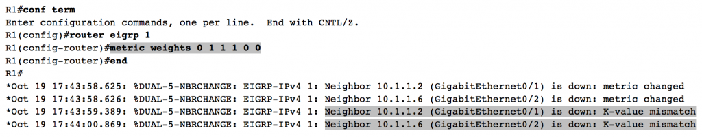
The first 0 in the metric weights 0 1 1 1 0 0 command seen in the above example specifies a TOS value of 0. The following five numbers set our five K-values: K1 = 1, K2 = 1, K3 = 1, K4 = 0, K5 = 0. This collection of K-values will now consider not just bandwidth and delay, but also load when performing a metric calculation. However, we have an issue. Notice the console messages appearing after our configuration. Both of our neighborships have been torn down, because router R1 now has different K-values than routers R2 and R3. Recall that EIGRP neighbors must have matching K-values, meaning that if you change the K-values on one EIGRP-speaking router, you need an identical set of K-values on each of its EIGRP neighbors. Once you configure matching K-values on those neighbors, then each of their neighbors need matching K-values. As you can see, in a large topology, there could be a significant administrative burden associated with K-value manipulation.
Successor and Feasible Successor Routes
One reason EIGRP rapidly converges in the event of a route failure is EIGRP often has a backup route standing by to take over if the primary route goes down. To make sure the backup route is not dependent on the primary route, EIGRP thoroughly vets the backup route by making sure it meets EIGRP’s feasibility condition. Specifically, the feasibility condition states:
An EIGRP route is a feasible successor route if its reported distance (RD) from our neighbor is less than the feasible distance (FD) of the successor route.
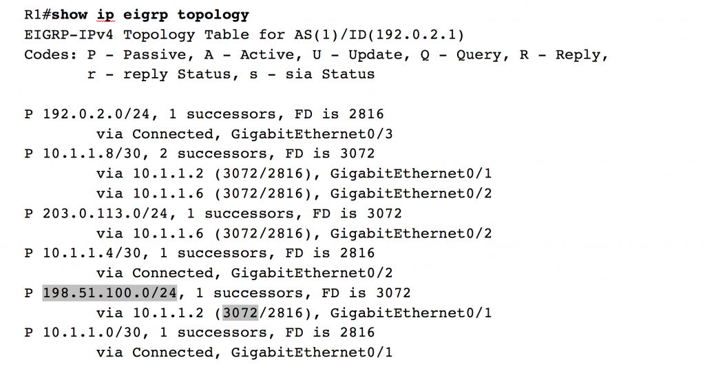
For example, consider the topology shown in the following figure and the corresponding configuration given the example below. Notice the 10.1.1.8 /30 network (between routers R2 and R3) is reachable from R1 via R2 or via R3. If router R1 uses the route via R2, it crosses a 1 Gbps link to reach the destination network. However, the route via R3 causes traffic to cross a slower 100 Mbps link. Since EIGRP considers bandwidth and delay by default, we can determine through observation that the preferred route is via router R2. However, what if the link between routers R1 and R2 goes down? Is there a feasible successor route that can almost immediately take over? Again, through observation, we might conclude that router R1 would use the feasible successor route via router R3. However, before we jump to that conclusion, we should confirm that the path via R3 meets the feasibility condition.
The Feasible Successor Condition Met on Router R1
Just by virtue of the fact that the route via router R3 (that is, via 10.1.1.6) appears in the output of the show ip eigrp topology command issued on router R1, we can conclude that the path via R3 is indeed a feasible successor route. However, let’s examine the output a bit more closely to determine why it’s a feasible successor route.
First, consider the entry from the output in the above example identifying the successor route (that is, the preferred route):
via 10.1.1.2 (3072/2816), GigabitEthernet0/1
The via 10.1.1.2 portion of the output says that this route points to a next-hop address of 10.1.1.2, which is router R2. The GigabitEthernet0/1 portion of the output indicates that we exit router R1 via the Gig 0/1 interface (that is, the egress interface). Now let’s examine those two numbers in parenthesis: (3072/2816). The value of 2816 is called the reported distance (RD). Some literature also refers to this value as the advertised distance (AD). These terms, which can be used synonymously, refer to the EIGRP metric reported (or advertised) to use by our EIGRP neighbor. In this instance, the value of 2816 is telling us that router R2’s metric (that is, distance) to network 10.1.1.8 /30 is 2816. The value of 3072 in the output is router R1’s feasible distance (FD). The FD is calculated by adding our neighbor’s RD to the metric required to reach our neighbor. Therefore, if we add the EIGRP metric between routers R1 and R2 to router R2’s RD, we get the FD (that is, the total distance) required for R1 to get to the 10.1.1.8 /30 via router R2. By the way, the reason router R1 determines the best path to the 10.1.1.8 /30 network is via via router R2 (that is, 10.1.1.2) as opposed to router R3 (that is, 10.1.1.6) is because the FD of path via R1 (3072) is less than the FD of the path via R2 (28,416).
Next, consider the entry for the feasible successor route from the above example:
via 10.1.1.6 (28416/2816), GigabitEthernet0/2
The via 10.1.1.6 portion of the output says this route points to a next-hop address of 10.1.1.6, which is router R3. The GigabitEthernet0/2 portion of the output indicates that we exit router R1 via the Gig 0/2 interface. This entry has an FD of 28,416 and an RD of 2816. However, before EIGRP just blindly considers this backup path a feasible successor, it checks the route against the feasibility condition. Specifically, the EIGRP process on router R1 asks if the RD from router R3 is less than the FD of the successor route. In this case, the RD from router R3 is 2816, which is indeed less than the successor’s FD of 3072. Therefore, the route via router R3 is considered a feasible successor route.
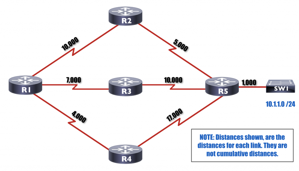
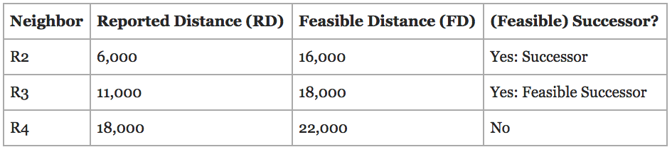
To reinforce this important concept just a bit more, consider the topology shown below. The EIGRP process on router R1 has learned three paths to reach the 10.1.1.0 /24 network. However, EIGRP next needs to determine which of those paths is the successor route, which (if any) of the paths are feasible successor routes, and which (if any) of the paths are neither a successor nor a feasible successor route. The results of EIGRP’s calculations are provided in the table below.
Feasible Successor Sample Calculations
Using the above table as a reference, first consider router R1’s path to the 10.1.1.0 /24 network via router R2. From router R2’s perspective, the distance to the 10.1.1.0 /24 network is the distance from R2 to R5 (which is 5,000) plus the distance from R5 out to the 10.1.1.0 /24 network (which is 1,000). This gives us a total of 6,000 for the distance from router R2 to the 10.1.1.0 /24 network. This is the distance router R2 reports to router R1. Therefore, router R1 sees an RD of 6,000 from router R2. Router R1, then adds the distance between itself and router R2 (which is 10,000) to the RD from R2 (which is 6,000) to determine its FD to reach network 10.1.1.0 /24 is 16,000 (that is, 10,000 + 6,000 = 16,000). The EIGRP process on router R1 perform similar calculations for paths to the 10.1.1.0 /24 network via routers R3 and R4. The following illustrates the calculations, which led to the values seen in the table.
![]()
Router R1 then examines the results of these calculations and determines that the shortest distance to the 10.1.1.0 /24 network is via router R2, because the path via R2 has the lowest FD (of 16,000). This path determined to have the shortest distance is deemed the successor route. Router R1 then attempts to determine if either of the other routes meet EIGRP’s feasibility condition. Specifically, router R1 checks to see of the RD from routers R3 or R4 is less than the FD of the successor route. In the case of R3, its RD of 11,000 is indeed less than the FD of the successor route (which is 16,000). Therefore, the path to the 10.1.1.0 /24 network via R3 qualifies as a feasible successor route. However, the route via R4 does not qualify, because R4’s RD of 18,000 is greater than 16,000 (the the FD of the successor route). As a result, the path to the 10.1.1.0 /24 network via router R4 is not considered to be a feasible successor route.
By the way, you can watch me teach EIGRP as part of the curriculum in the following video courses:
CCNA R/S (200-125) Complete Video Course
CCNP ROUTE (300-101) Complete Video Course
That’s going to wrap it up for our second installment in the Understanding EIGRP series. In the next post of this series, we’ll be examining EIGRP timers (which act quite differently than OSPF timers).
By the way, if you missed the first post in this series, you can check it out here:
See you next time!

Kevin Wallace, CCIEx2 (R/S and Collaboration) #7945